BioCHP plant module
The BioCHP plant module incorporates the following mass/energy streams and unit process operations:
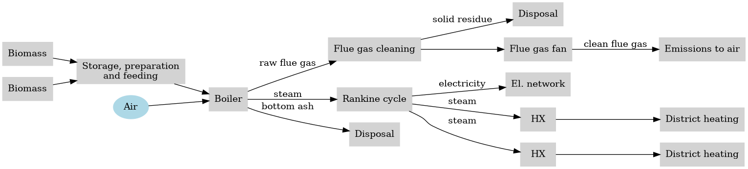
The model includes the following main processes:
- Supply, storage and handling of the solid biomass,
- Combustion of the biomass with recovery of the combustion heat for production of superheated steam,
- Direct utilization of the steam for production of electricity in a steam turbine,
- Production of heat through extractions from the steam turbine, and
- Cleaning of the raw flue gas after combustion to remove particulate matter, acid gases and volatile organic components.
The capacity of the bioCHP plant is defined in terms of the total power output from the biomass boiler, calculated from the electric power and heat demands. The model considers two sold residues, i.e., bottom ash from the boiler and residue from flue gas cleaning containing fly ash and consumed lime.
Important features of the model include:
- The feedstock is defined as a mixture of several types of Biomass resources.
- Multiple heat demands are specified by thermal power, temperature, and pressure for district heating (each through a heat exchanger) or as direct steam export.
The module is implemented as a nonlinear C++ model. It allows for multiple different configurations. It is not directly linked to EnergyModelsX. Instead, a sampling routine for capturing both the costs (capital expenditures and operating expenses) as well as the performance (heat-to-power production and varying power levels) will be implemented in a later stage. This sampling routine allows a tight integration of the model within the EnergyModelsX framework.
Parameters
The parameters of the BioCHP plant model can be differentiated into external inputs and internal parameters as defined below.
Inputs
The first relevant input category is related to the biomass used in the CHP plant. The biomass is included in the module through a combination of strings. It is hence necessary to use the strings specified within the module. The following input is required for the biomass feed:
- none (
fuel_defin the model asvector[string]): The type of biomass. Multiple biomass types can be provided to the module, e.g.,spruce_bark.
The currently implemented feedstock strings arespruce_stem,spruce_bark,spruce_T&B, andbirch_stem. - \( Y_j^F \) (
Y_fuel[j]in the model asvector[double]): The mass fraction of biomass resource \( j \) in the feed. The total mass fraction must sum to 1. - \( Y_{H_2O,j}^F \) (
YH2O_fuel[j]in the model asvector[double]): The moisture content of biomass resource \( j \) as a mass fraction. It corresponds to the water content in the total wet mass.
In addition, the input for the desired plant characteristics must be provided. This input can be specified by the user through a text file, although upper bounds may exist for some variables. The following input is required for the plant characteristics:
- \( T_{h,k} \) (
T_h[k]in the model asvector[double]): The temperature level of heat demand \( k \) in °C. As the CHP plant can provide heat at several temperature levels, it is possible to specify them directly. - \( P_{h,k} \) (
P_h[k]in the model asvector[double]): The outlet pressure of heat demand \( k \) in bar gauge. (Provide the pressure by subtracting the ambient pressure. The combination of temperature and pressure determines whether the heat is supplied as steam or as hot water.) - \( \dot{Q}_{k} \) (
Q_h[k]in the model asvector[double]): The heat demand at the individual temperature and pressure levels \( k \) in MW. - \( \dot{W}_{el} \) (
W_elin the model asdouble): The electric power output of the CHP plant in MW.
- Note
- Vector positions: Both the input biomass and heat demands are specified as vectors. This implies that the ordering of the biomass types, their mass fractions, and the moisture content requires correct indexing. Similarly, the thermal power, temperature, and pressure conditions of the heat demands must follow the correct indexing.
Internal
The different biomass types furthermore have a set of internal parameters. These parameters describe the characteristics of the biomass that are fundamental properties of the respective biomass. Adding a new type of biomass requires adding the following parameters:
- \( Y_{i,j}^F \) (
Yi.fuel[j]in the model): The atomic composition of biomass \( j \) in kg/kg dry basis, i.e., without any water content. - \( Y_{ash,j}^F \) (
Yash.fuel[j]in the model): The ash content in biomass \( j \) (kg/kg dry basis). - \( LHV_j^F \) (
LHV.fuel[j]in the model): The lower heating value of biomass \( j \) in MJ/kg. - \( x \): The hydrogen-to-carbon atomic molar ratio.
- \( y \): The oxygen-to-carbon atomic molar ratio.
Furthermore, process characteristics can be specified internally:
- \( \lambda_{air}^{comb} \) (
lambda_combin the model): The excess air in the combustion process (-). - \( T_{stm}^{boiler} \) (
T_stmin the model): The Boiler steam temperature in °C. - \( P_{stm}^{boiler} \) (
P_stmin the model): The Boiler steam pressure in bar gauge. - \( \eta_S^{ST_n} \) (
eta_s[n]in the model): The isentropic efficiency for steam turbine stage \( n \). (Individual steam turbines of the Rankine cycle can have different isentropic efficiencies.)
- Note
- Format of the parameters: All internal parameters are required as
doubletypes in the model.
Outputs (standard)
- \( \dot{M}_F \) (
M_fuel): biomass mass flow rate (kg/s) - \( \dot{H}_F \) (
H_fuel): energy flow rate of biomass (MW) - \( C_{inv} \) (
C_inv): capital expenditures (M$) - \( C_{op,d} \) (
C_op_d): annual variable OPEX (M$) - \( C_{op,f} \) (
C_op_f): annual fixed OPEX (M$)
\tip All outputs are required to be double type.
Outputs (standard)
The standard output of the model is given as
- \( \dot{M}_F \) (
M_fuelin the model) is the input mass flow rate of biomass to the BioCHP plant in kg/s. - \( \dot{H}_F \) (
H_fuelin the model) is the input energy flow rate of biomass to the BioCHP plant in MW. - \( C_{inv} \) (
C_invin the model) represents the capital expenditures in M$. - \( C_{op,d} \) (
C_op_din the model) represents the annual direct variable operating expenses in M$.
It is assumed that the plant operates at XXX h/year at full capacity. - \( C_{op,f} \) (
C_op_fin the model) represents the annual fixed operating expenses in M$.
- Note
- Format of the outputs: All outputs are required as
doubletypes in the model.
Mathematical formulation
Mass and energy flows (nominal steady state operation)
Considering
- a biomass mixture defined by the mass fraction of each type of feedstock in the mixture \( Y_j^F \),
- the net power production from the Rankine cycle \( \dot{W}_{el}^{RK} \), and
- the external heat demands \( \dot{Q}_{k} \)
as inputs, the total energy rate of the input biomass to the CHP plant \( \dot{H}_F \) with \( N_q \) steam extractions to cover heat demands is calculated as
\[ \dot{W}_{el}^{RK} = \sum_{n=0}^{N_q} \left(\dot{H}_F \frac{(q_{stm}^{boiler}/h_{fuel})}{(h_{stm}^{boiler}-h_{bfw}^{boiler})} - \sum_{k=0}^n \frac{\dot{Q}_{k}}{(h_{stm}^{k}-h_{o}^{k})} \right) (h_{in}^{ST_n}-h_{out,s}^{ST_n})\eta_S^{ST_n} \]
with
\[ q_{stm}^{boiler} = \frac{h_{fuel} - h_g^{FGC} - h_{ba}^{boiler} - h_{s}^{FGC}}{(1-q_{loss})}, \]
that is, the difference in mass enthalpy between the biomass fuel and the output from the system (i.e. the flue gas, the fly ash, and the bottom ash).
The value \( q_{loss} \) corresponds in this situation to the fraction of heat loss.
The specific enthalpy of the fuel is calculated through the lower heating values of the individual biomass resources (indexed through \( j \)), excluding the moisture in the resources (indexed through \( H_2O \)):
\[ h_{fuel} = \sum_j Y_j^F\Big[(1-Y_{H_2O,j})\, LHV_j - Y_{H_2O,j}\, h_{v,H_2O}\Big] \]
The specific enthalpy of the combustion gas is calculated through the difference between its temperature and the reference temperature \( T_0 \), the heat capacities \( c_{p,g,j} \) and
\[ h_g^{FGC} = (T_g^{FGC}-T_0) \sum_j \Big\{ Y_j^F\, c_{p,g,j} \Big( Y_{H2O,j} + (1-Y_{H2O,j})\Big[ 1+\lambda_{air}^{comb}\, Y_{C,j}\Big(\frac{W_{air}}{W_C}\Big)(1+x/4-y/2)\Big]\Big) \Big\} \]
Here, \( W_{air} \) and \( W_C \) are the molecular weight of air (28 g/mol) and the atomic weight of carbon (12 g/mol).
The specific enthalpy of the bottom ash is given by
\[ h_{ba}^{boiler} = \Big[c_{ba}\,(T_{ba}^{boiler}-T_0) + Y_{C,ba}\, h_C\Big]\, f_{ba}\,\sum_j \Big[ \dot{Y}_j^F\,(1-Y_{H2O,j})\, Y_{ash,j}^F \Big] \]
and the specific enthalpy of the flue gas per unit mass feedstock is given by
\[ h_{s}^{FGC} = (T_{s}^{FGC}-T_0) \Big[ m_{lime}\, c_{lime} + f_{fa}\, c_{fa}\,\sum_j \dot{Y}_j^F\,(1-Y_{H2O,j})\, Y_{ash,j}^F \Big] \]
- Note
- Specific enthalpies: All specific enthalpies described above are relative to the mass flow of the biomass feedstock \( \dot{M}_F \).
Using the calculated value for \( \dot{H}_F \), other material and energy flows for the BioCHP plant are calculated:
- Mass flow rate of the biomass mixture and of each feedstock \( j \):
\[ \begin{aligned} \dot{M}_F & = \dot{H}_F/h_{fuel} \\ \dot{M}_j^F & = \dot{M}_F \sum_{j=1}^{N_j} Y_j^F \\ \end{aligned} \]
- Mass flow rate and energy flow rate of bottom ash ( \( ba \)) from the boiler:
\[ \begin{aligned} \dot{M}_{ba}^{boiler} & = \dot{M}_F \,(1+Y_{C,ba})\, f_{ba}\, \sum_j \Big[ Y_{ash,j}^F\, \dot{Y}_j^F\,(1-Y_{H2O,j}) \Big] \\ \dot{H}_{ba}^{boiler} & = \dot{M}_F\, h_{ba}^{boiler} \\ \end{aligned} \]
- Inlet mass flow rate of lime to flue gas cleaning:
\[ \dot{M}_{lime} = \dot{M}_F\, m_{lime,b}\, \sum_j \frac{Y_{S,j} + Y_{Cl,j}}{Y_{S,b}+Y_{Cl,b}} \]
- Mass flow rate and energy flow rate of solid residue ( \( s \)) from the flue gas cleaning:
\[ \begin{aligned} \dot{M}_{s}^{FGC} & = \dot{M}_F \Big[ m_{lime} + f_{fa}\, \sum_j \dot{Y}_j^F\,(1-Y_{H2O,j})\, Y_{ash,j}^F \Big] \\ \dot{H}_{s}^{FGC} & = \dot{M}_F\, h_{s}^{FGC} \\ \end{aligned} \]
- Mass and energy flow rates of flue gas from the CHP plant:
\[ \begin{aligned} \dot{M}_{g}^{FGC} & = \dot{M}_F\, \sum_j \dot{Y}_j^F\Big[ Y_{H2O,j} + (1-Y_{H2O,j})\Big( 1+\lambda_{air}^{comb}\, Y_{C,j}\Big(\frac{W_{air}}{W_C}\Big)(1+x/4-y/2)\Big) \Big] \\ \dot{H}_{g}^{FGC} & = \dot{M}_F\, h_g^{FGC} \\ \end{aligned} \]
- Thermal energy and mass flow rates of steam ( \( stm \)) produced from the boiler:
\[ \begin{aligned} \dot{Q}_{stm}^{boiler} & = \frac{\dot{H}_{fuel} - \dot{H}_g^{FGC} - \dot{H}_{ba}^{boiler} - \dot{H}_{s}^{FGC}}{(1-q_{loss})} \\ \dot{M}_{stm}^{boiler} & = \frac{\dot{Q}_{stm}^{boiler}}{(h_{stm}^{boiler}-h_{bfw}^{boiler})} \\ \end{aligned} \]
CAPEX
The installed cost of equipment \( k \) is calculated from
\[ C_{eq,k} = C_{P,k}^B \left(\frac{S_k}{S_k^B}\right)^{n_k} \left(\frac{I}{I_B}\right) f_{inst,k}, \]
where \( C_{P,k}^B \) is the purchase cost for a base-case equipment size \( S_k^B \) in the reference year, \( S_k \) is the actual equipment size, \( n_k \) is the equipment scale factor, and \( f_{inst,k} \) is the installation factor. The ratio \( I/I_B \) is the price index ratio between the actual year and the reference year (e.g. using the Chemical Engineering Plant Cost Index).
The following equipment cost parameters are used:
| Equipment | S_k^B | C_{P,k}^B (M$) | f_{inst,k} | n_k | Base year |
|---|---|---|---|---|---|
| Biomass storage and preparation | 25 t/h | 5.4 | 2.1 | 0.5 | 2007 |
| Biomass boiler | 25 t/h | 7.9 | 2.1 | 0.7 | 2007 |
| Flue gas cleaning | 67 t/h | 0.18 | 2.7 | 0.7 | 2007 |
| Steam turbines and condenser | 1500 MW | 40.5 | 1.3 | 0.7 | 2006 |
| Heat Exchanger (heat export) | 100 m² | 0.086 | 2.8 | 0.71 | 2012 |
The total equipment cost is then given by
\[ C_{eq} = \sum_k C_{eq,k} \]
The total capital expenditures (CAPEX) is evaluated in terms of the total permanent investment \( C_{inv} \) from:
\[ C_{inv} = \sum_k C_{eq,k}\,(1+f_{pip}+f_{el}+f_{I\&C})\Big[(1+f_{site}+f_{building})+f_{com}\Big](1+f_{cont,k}+f_{eng,k})(1+f_{dev}) \]
where \( C_{eq,k} \) denotes the installed cost of equipment and the \( f_i \) are cost parameters defined as follows:
- \( f_{pip} = 0.065 \) for interconnecting piping between equipment,
- \( f_{el} = 0.05 \) for the plant electric system,
- \( f_{I\&C} = 0.05 \) for the instrumentation and control system,
- \( f_{site} = 0.17 \) for land and site preparation,
- \( f_{building} = 0.20 \) for construction of buildings,
- \( f_{com} = 0.10 \) for commissioning,
- \( f_{dev} = 0.02 \) for project development and licenses,
- \( f_{eng,k} = 0.15 \) for engineering, and
- \( f_{cont,k} = 0.20 \) for contingency.
OPEX
The OPEX is defined as the total annual operating costs calculated from
\[ C_{op} = C_{op,d} + C_{op,f}, \]
where:
- \( C_{op,d} \) denotes the variable operating cost, proportional to the annual operating time \( t_{op} \), including the
- supply of biomass (unit price: 100 $/t),
- purchase of lime (unit cost: 0.25 $/kg),
- disposal of flue gas cleaning solid residue (unit cost: 40.0 $/t), and
- disposal of bottom ash (unit cost: 20.0 $/t).
- \( C_{op,f} \) denotes the fixed operating costs required for keeping the BioCHP plant in operation, including:
- Maintenance cost:
\[ C_{maint} = 0.05\, C_{eq} \]
- Insurance:
\[ C_{ins} = 0.01\, C_{inv} \]
- Administration and site services:
\[ C_{adm} = 0.03\, C_{inv} \]
- Labor cost:
\[ C_{labor} = \sum_k N_k^{labor}\, c_{b,k}^{labor}\,\Big[1+f_{oh,k}^{labor}\Big] \]
Here, the subscript \( k \) denotes the personnel categories and the parameters are defined as follows:
1) Plant manager:
\[ \begin{aligned} c_{b,k}^{labor} & = 162~k\$/year \\ N_k^{labor} & = 1 \\ f_{oh,k}^{labor} & = 0.0 \\ \end{aligned} \]
2) O&M manager:
\[ \begin{aligned} c_{b,k}^{labor} & = 96~k\$/year \\ N_k^{labor} & = \begin{cases} 1 ,& \text{if} ~ \dot{M}_F < 10~\text{t/h} \\ 2 ,& \text{if} ~ \dot{M}_F > 10~\text{t/h} \\ \end{cases} \\ f_{oh,k}^{labor} & = 1.2 \\ \end{aligned} \]
3) O&M engineer:
\[ \begin{aligned} c_{b,k}^{labor} & = 88~k\$/year \\ N_k^{labor} & = \begin{cases} 1 ,& \text{if} ~ \dot{M}_F < 10~\text{t/h} \\ 2 ,& \text{if} ~ \dot{M}_F > 10~\text{t/h} \\ \end{cases} \\ f_{oh,k}^{labor} & = 1.2 \\ \end{aligned} \]
4) Shift operator:
\[ \begin{aligned} c_{b,k}^{labor} & = 37~k\$/year \\ N_k^{labor} & = \begin{cases} 3 ,& \text{if} ~ \dot{M}_F < 10~\text{t/h} \\ 6 ,& \text{if} ~ \dot{M}_F > 10~\text{t/h} \\ \end{cases} \\ f_{oh,k}^{labor} & = 1.3 \\ \end{aligned} \]
- Note
- Number of employees: The number of employees depends on the size of the plant. The chosen distinction is based on the mass flow of biomass into the plant \( \dot{M}_F \), with a change in staffing when the flow exceeds 10 t/h.
File structure
bioCHP.cpp contains the C++ function to interface with EMX.
It has the following structure:
├── Definitions.h
├── Costs.h
├── Flows
│   ├── Flow_definitions.h
│   ├── Flow_calculations.h
│   └── Thermodynamics
│       └── Water_thermodynamics.h
└── Processes
    ├── bioCHP_plant.h
    ├── Combustion.h
    ├── Rankine_cycle.h
    └── Flue_gas_cleaning.h